Motion Relationships
Syllabus mapping
PY-11-01 — Fundamentals of Mechanics. Covers: constructing and interpreting displacement–time, velocity–time and acceleration–time graphs; relating gradient and area under these graphs to other quantities of motion; the equations for uniformly accelerated motion (SUVAT); relative velocity in two dimensions.
Wording above is paraphrased for teaching use — cross-check against the official syllabus PDF (see Resources) before treating any line as verbatim NESA text.
You need to know: how to read and build the three motion graphs, how gradient and area connect them to each other, how to pick and use the right SUVAT equation, and how to combine velocities in two dimensions.
Assumed knowledge check
Before this page makes sense, you should be comfortable with:
- Graphs — reading/constructing line graphs, gradient, area under a graph
- Algebra — rearranging multi-step equations
- Quantities of Motion — scalar/vector distinction and vector addition, both used again here
Core
The three motion graphs
| Graph | Gradient gives | Area under gives |
|---|---|---|
| Displacement–time | Velocity | — (not used) |
| Velocity–time | Acceleration | Displacement |
| Acceleration–time | — (rate of change of acceleration, not examined here) | Change in velocity |
Read these graphs the same way every time: gradient = rate of change, area = the thing being accumulated. A steeper displacement–time graph means a larger velocity; a flat velocity–time graph (gradient zero) means zero acceleration, not zero velocity — a very common mix-up.
Worked example
A velocity–time graph shows an object accelerating uniformly from \(0\) to \(8\ \text{m s}^{-1}\) over \(4\ \text{s}\), then travelling at constant \(8\ \text{m s}^{-1}\) for a further \(3\ \text{s}\).
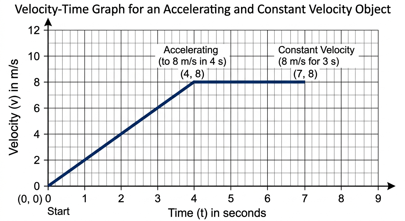
Acceleration during the first phase (gradient of the v–t graph):
Total displacement (area under the v–t graph — a triangle plus a rectangle):
SUVAT equations
For motion with uniform (constant) acceleration only. These three are given on your HSC data sheet, written exactly as shown there (note the vector arrows — they're not just decoration, they signal these are vector equations valid in any direction, not only "forwards"):
where \(s\) = displacement, \(u\) = initial velocity, \(v\) = final velocity, \(a\) = acceleration, \(t\) = time. The third equation drops the arrows because it relates magnitudes, not directions.
Each is missing exactly one of the five variables — pick the equation missing the variable you don't have and don't need:
| Equation | Missing variable | On data sheet? |
|---|---|---|
| \(\vec{v} = \vec{u} + \vec{a}t\) | \(s\) | Yes |
| \(\vec{s} = \vec{u}t + \tfrac{1}{2}\vec{a}t^2\) | \(v\) | Yes |
| \(v^2 = u^2 + 2as\) | \(t\) | Yes |
| \(s = \tfrac{1}{2}(u+v)t\) | \(a\) | No — see note below |
A fourth equation you'll see in textbooks — but not on the data sheet
\(s = \tfrac{1}{2}(u+v)t\) is genuinely useful (handy whenever \(a\) isn't given or needed) and it's easy to derive from the two vector equations above, but NESA doesn't print it. Don't plan on it being handed to you in the exam — either derive it on the spot from the two you are given, or pick a different equation for that problem. Worked derivation is in the Extension box below.
Worked example
A car accelerates uniformly from rest at \(3\ \text{m s}^{-2}\) for \(5\ \text{s}\). Find the distance travelled.
Known: \(u = 0\), \(a = 3\ \text{m s}^{-2}\), \(t = 5\ \text{s}\). Unknown and not needed: \(v\). Use the equation missing \(v\):
Relative velocity in 2D
The velocity of A relative to B is the vector difference:
Since this is a vector subtraction, use the component method from Quantities of Motion: reverse \(\vec{v}_B\)'s components and add.
Worked example
A boat travels at \(\vec{v}_{boat} = 5\ \text{m s}^{-1}\) east relative to the water. The water itself flows at \(\vec{v}_{water} = 2\ \text{m s}^{-1}\) north relative to the bank. Find the boat's velocity relative to the bank.
This is vector addition, not subtraction (the boat's velocity relative to the bank is its velocity relative to the water, plus the water's velocity relative to the bank):
Components: \(v_x = 5\ \text{m s}^{-1}\) (east), \(v_y = 2\ \text{m s}^{-1}\) (north).
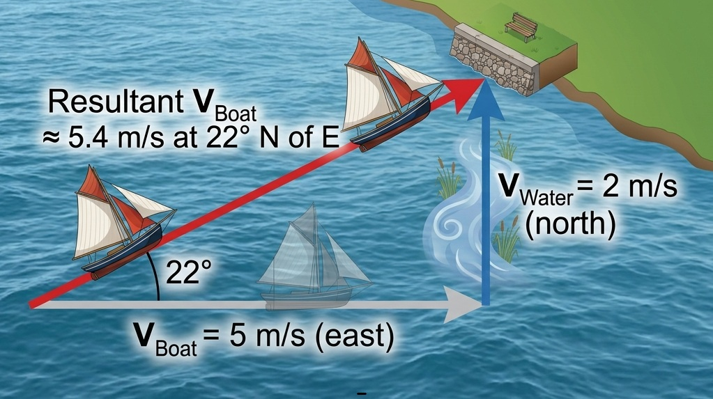
Note this specific example is an addition, not the general \(\vec{v}_{AB}=\vec{v}_A-\vec{v}_B\) subtraction defined above — the two velocities here are already relative to a common middle reference (the water), so they combine directly rather than needing one reversed.
Practical
Suggested prac: two independent methods of determining g experimentally, e.g. (1) timing free-fall over a measured drop height and using \(s = \tfrac{1}{2}gt^2\), and (2) a simple pendulum using \(T = 2\pi\sqrt{L/g}\) rearranged for \(g\). TODO — link this school's actual prac instructions once written; the two-methods comparison is also a natural spot to discuss experimental uncertainty (see Working Scientifically: Precision and Uncertainty) — the pendulum method's \(T^2\) vs \(L\) graph is also the worked example on Working Scientifically: Representing Data.
Advanced
Non-uniform acceleration on a v–t graph. SUVAT only applies when acceleration is constant. When it isn't, the graph's gradient changes over time, and total displacement still equals the area under the curve — but that area may need to be split into geometric shapes (as in the worked example above) or, for a curved graph, estimated using the trapezoidal rule / counting squares. The same logic examiners test with a-t graphs: area under an a–t graph gives change in velocity, even when acceleration itself is changing.
Multi-stage SUVAT problems — e.g. an object thrown upward that decelerates, stops, then reverses — need each stage (up, then down) treated as a separate uniformly-accelerated phase with its own \(u\), \(v\), \(t\), taking care with the sign convention for direction.
Extension
Beyond the Physics 11–12 syllabus — won't appear in the HSC, included for interest / depth study inspiration.
📎 Depth study idea
The SUVAT equations aren't arbitrary — they fall straight out of calculus, as flagged in Quantities of Motion. Starting from constant acceleration \(a\):
\(v^2 = u^2 + 2as\) then follows by eliminating \(t\) between the two. This is the natural next step for a student who found the calculus connection in Quantities of Motion interesting, and generalises directly to non-uniform acceleration (Advanced, above) once \(a\) is written as a function of \(t\) rather than a constant — worth a depth study if a student wants to handle a specific non-constant-acceleration scenario properly (e.g. drag-affected motion) rather than approximating from a graph.
Deriving the "missing" fourth equation. Since acceleration is constant, velocity increases linearly with time, so the average velocity over the interval is just the mean of the start and end values:
Displacement is average velocity times time, giving exactly the equation the data sheet doesn't print:
Video/visual resources
- 🖥️ PhET Simulation — Moving Man — embedded on Quantities of Motion, also directly relevant to the graph relationships above
Khan Academy — building and choosing the SUVAT equations
Four short videos (external links, they open on khanacademy.org) that build the SUVAT equations straight out of a v–t graph and then show how to pick between them — the same logic as the SUVAT equations section above. Listed in Khan Academy's own learning-sequence order:
- 🎥 Khan Academy — Deriving motion from v–t graphs — gets the three data-sheet equations from the graph's gradient and area
- 🎥 Khan Academy — Intro to motion with constant acceleration
- 🎥 Khan Academy — Average velocity for constant acceleration — the \(s = \tfrac{1}{2}(u+v)t\) result from the Extension box
- 🎥 Khan Academy — Choosing kinematic equations — picking the equation by the variable you don't have and don't need
Physics High (NSW-syllabus-aligned, external links to YouTube)
- 🎥 Physics High — The equations of motion — single-video overview of the SUVAT material above, followed by 🎥 a worked example applying them
- 🎥 Physics High — Understanding Vectors — vector addition, the tool used for relative velocity below (also linked from Quantities of Motion)
Relative velocity in 2D (Physics High)
- 🎥 Physics High — Relative motion explained — the concept
- 🎥 Physics High — Sample worked relative motion problem — matches the river/boat-style worked example above
- 🖥️ Physics High — Relative motion interactive — explore two velocities combining, in your browser
Check yourself
-
A velocity–time graph shows constant deceleration from \(20\ \text{m s}^{-1}\) to \(0\) over \(10\ \text{s}\). Find (a) the acceleration and (b) the distance travelled.
Answer
(a) \(a = \dfrac{\Delta v}{\Delta t} = \dfrac{0 - 20}{10} = -2\ \text{m s}^{-2}\)
(b) Area under the graph (triangle): \(s = \tfrac{1}{2} \times 10 \times 20 = 100\ \text{m}\)
-
A stone is dropped from rest and falls for \(2.5\ \text{s}\) before hitting the ground. Taking \(g = 9.8\ \text{m s}^{-2}\), find the height it fell from.
Answer
Known: \(u = 0\), \(a = 9.8\ \text{m s}^{-2}\), \(t = 2.5\ \text{s}\), missing \(v\) (not needed).
\(s = ut + \tfrac{1}{2}at^2 = 0 + \tfrac{1}{2}(9.8)(2.5)^2 \approx 30.6\ \text{m}\)
-
Two cars travel on a straight road: Car A at \(25\ \text{m s}^{-1}\) east, Car B at \(15\ \text{m s}^{-1}\) east. Find Car A's velocity relative to Car B.
Answer
\(\vec{v}_{AB} = \vec{v}_A - \vec{v}_B = 25 - 15 = 10\ \text{m s}^{-1}\) east — from Car B's point of view, Car A pulls away at \(10\ \text{m s}^{-1}\).